
Photo by Creative Commons Attribution Share-Alike (CCYYSA)
import numpy as np
import pandas as pd
Introduction
Linear regression is a powerful and widely used statistical technique that allows us to model and analyze the relationship between a dependent variable and one or more independent variables. At its core, linear regression seeks to find the best-fitting line through a set of data points, minimizing the sum of the squared differences between the observed and predicted values. This best-fit line can be used for prediction, inference, and understanding the underlying patterns in the data.
In the realm of linear algebra, the process of finding the best-fitting line in linear regression can be elegantly expressed and solved using matrix operations. One of the most efficient methods for solving linear regression is through matrix inversion, specifically by applying the Ordinary Least Squares (OLS) approach. This method leverages the power of matrix algebra to derive a closed-form solution for the coefficients that define the best-fitting line.
The key advantage of using matrix inversion in linear regression lies in its computational efficiency and clarity. By representing the linear regression model in matrix form, we can capture the relationships between variables and utilize matrix operations to solve for the coefficients. This approach not only simplifies the computational process but also provides a clear mathematical framework for understanding the solution.
This guide aims to provide a comprehensive introduction to solving linear regression using matrix inversion. We will explore the fundamental concepts of linear regression, delve into the mathematical formulation of the problem, and demonstrate how matrix inversion is applied to obtain the solution. By the end of this guide, you will have a solid understanding of how to leverage matrix algebra to solve linear regression problems efficiently and effectively.
Theory Background
Linear regression is a statistical method that models the relationship between a dependent variable and one or more independent variables. The goal is to find the best-fit line (or hyperplane in higher dimensions) that minimizes the discrepancies between the observed data points and the predicted values. This technique is widely used in fields such as economics, biology, engineering, and machine learning due to its simplicity and interpretability.
Mathematical Formulation
In the context of linear regression, the relationship between the dependent variable $y$ and the independent variables $x$ can be expressed as:
$$y = \beta X + \epsilon $$ *where:* * $y$ is the vector of observed values. * $X$ is the data matrix that includes a column of ones (for the intercept) and columns for each of the independent variables. * $β$ is the vector of coefficients that we aim to estimate. * $ϵ$ is the vector of errors or residuals.
Ordinary Least Squares Estimation (OLS)
The method of ordinary least squares or OLS aims to estimate the coefficients $β$ by minimizing the sum of the squared residuals:
$$min_{\beta} \sum_{i=1}^{n} (y_i – X_i \beta)^2$$This optimization problem can be solved analytically using matrix algebra. By taking the derivative of the sum of squared residuals with respect to $β$ and setting it to zero, we derive the normal equations:
$$X^TX\beta = X^Ty$$**Solving the Normal Equations**
The solution to the normal equations provides the OLS estimator for the coefficients $β$:
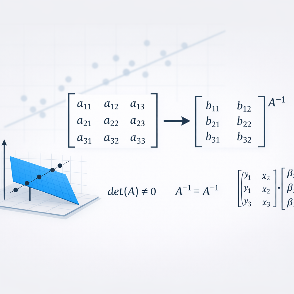
$$\beta = (X^TX)^{-1}X^Ty$$where:
- $X^T$ is the transpose of the matrix $X$, and
- $(X^TX)^{-1}$ is the inverse of the matrix $(X^TX)^{-1}$
Conditions for Matrix Inversion
Not all matrices are invertible. For the matrix $X^TX$ to have an inverse, the following conditions must be met:
- $X$ must be of full rank, meaning that its columns are linearly independent.
- $X^TX$ must be non-singular, which implies that it has a non-zero determinant.
- $X$ must be a square matrix.
Matrix Inverse Revisited
The inverse of a matrix $A$ is $A^{-1}$ such that $A * A^{-1} = I$ where $I$ is the identity matrix. Let
$$A = \begin{bmatrix} 1 & 0 & 0\\ -1 & 1 & 0\\ 0 & -1 & 1 \end{bmatrix}$$Then:
$$[A * I] = \begin{bmatrix} \begin{array}{ccc|ccc} 1 & 0 & 0 & 1 & 0 & 0 \\ -1 & 1 & 0 & 0 & 1 & 0 \\ 0 & -1 & 1 & 0 & 0 & 1 \\ \end{array} \end{bmatrix}$$Performing elementary row operations:
$$ ⇒ \begin{bmatrix} \begin{array}{ccc|ccc} 1 & 0 & 0 & 1 & 0 & 0 \\ 0 & 1 & 0 & 1 & 1 & 0 \\ 0 & -1 & 1 & 0 & 0 & 1 \\ \end{array} \end{bmatrix}$$
$$[I * A^{-1}] = \begin{bmatrix} \begin{array}{ccc|ccc} 1 & 0 & 0 & 1 & 0 & 0 \\ 0 & 1 & 0 & 1 & 1 & 0 \\ 0 & 0 & 1 & 1 & 1 & 1 \\ \end{array} \end{bmatrix}$$
Therefore, the inverse of matrix $A$ is
$$A^{-1} = \begin{bmatrix} 1 & 0 & 0\\ 1 & 1 & 0\\ 1 & 1 & 1 \end{bmatrix}$$Pseudoinverse of a Matrix
The pseudoinverse is a generalization of the inverse matrix. It is especially useful for matrices that are not square or do not have a regular inverse. For a given matrix $A$, the pseudoinverse $A^{+}$ satisfies the following properties:
- $AA^+ = A$
- $A^+AA^+ = A^+$
- $(AA^+)^T = AA^+$
- $(A^+A)^T = A^+A$
To find the pseudoinverse $A^{+}$, use the Singular Value Decomposition or SVD method.
- Compute the SVD of A. $A = U*Σ*V^T$
- Compute for the pseudoinverse $Σ^+$ of the diagonal matrix $Σ$.
- Form the pseudoiverse $A^+ = VΣ^+U^T$.
Interactive Visuals
Here are some sites that show interactive visuals on linear regression:
Interactive 3d Regression Tool
Interactive Visualization of Linear Regression
Inverse Matrix With Regression
Applications in Machine Learning
Linear regression forms the foundation of many machine learning algorithms and is often used for predictive modeling. Understanding the theory and application of matrix inversion in linear regression is crucial for building more complex models and for performing feature engineering and data preprocessing.
Predicting House Prices
Real estate companies and prospective homebuyers often want to predict the prices of houses based on various features like the size of the house, number of bedrooms, location, etc. The dataset contains historical data of house prices along with features such as:
- size (in square feet)
- number of bedrooms
- number of bathrooms
- location (encoded as numerical features)
- year built
- lot size
Code
# Sample dataset
data = {
    'size': [1500, 2000, 2500, 1800, 2200],
    'bedrooms': [3, 4, 4, 3, 3],
    'bathrooms': [2, 3, 3, 2, 2],
    'location': [1, 2, 2, 1, 2],  # Encoded location
    'price': [300000, 400000, 450000, 350000, 420000]
}

df = pd.DataFrame(data)

# Feature matrix X and target vector y
X = df[['size', 'bedrooms', 'bathrooms', 'location']]
X.insert(0, 'intercept', 1)  # Add the intercept column at the first column
y = df['price']

# Convert to numpy arrays
X = np.array(X)
y = np.array(y)

# Calculate the OLS coefficients or beta
X_transpose = np.transpose(X)
beta = np.linalg.inv(X_transpose @ X) @ X_transpose @ y # See formula for beta in Theory Section

# Print the estimated coefficients
print("Estimated coefficients:", beta)

# Example prediction for a new house
new_house = np.array([1, 2000, 3, 2, 1])
predicted_price = new_house @ beta
print("Predicted price for the new house:", predicted_price)
This model will use the historical data to learn the relationship between house features and prices. The estimated coefficients $β$ can then be used to predict the price of a new house based on its features.
# @title
# Code

# Sample dataset
data = {
    'size': [1500, 2000, 2500, 1800, 2200],
    'bedrooms': [3, 4, 4, 3, 3],
    'bathrooms': [2, 3, 3, 2, 2],
    'location': [1, 2, 2, 1, 2],  # Encoded location
    'price': [300000, 400000, 450000, 350000, 420000]
}

df = pd.DataFrame(data)

# Feature matrix X and target vector y
X = df[['size', 'bedrooms', 'bathrooms', 'location']]
X.insert(0, 'intercept', 1)  # Add the intercept column at the first column
y = df['price']

# Convert to numpy arrays
X = np.array(X)
y = np.array(y)

# Calculate the OLS coefficients or beta
X_transpose = np.transpose(X)
beta = np.linalg.inv(X_transpose @ X) @ X_transpose @ y # See formula for beta in Theory Section

# Print the estimated coefficients
print("Estimated coefficients:", beta)

# Sample prediction for a new house
new_house = np.array([1, 2000, 3, 2, 1])
predicted_price = new_house @ beta
print("Predicted price for the new house:", predicted_price)
Estimated coefficients: [-4.27628676e+05  2.88604454e+02  3.15091912e+05 -5.71875000e+04
  3.02941176e+04]
Predicted price for the new house: 1010775.0847252901
Code Walkthrough
The code above can be summarized in the following steps:
- Load the data.
- Create the feature matrix X and insert the intercept column at the first column.
- Create the target vector Y.
- Compute for the Ordinary Least Squares (OLS) coefficients or $β$.
- Predict new data point.
Loading the Data
    data = {
      'size': [1500, 2000, 2500, 1800, 2200],
      'bedrooms': [3, 4, 4, 3, 3],
      'bathrooms': [2, 3, 3, 2, 2],
      'location': [1, 2, 2, 1, 2],  # Encoded location
      'price': [300000, 400000, 450000, 350000, 420000]
    }
    df = pd.DataFrame(data)
Data contains information about the size of the house, number of bedrooms, number of bathrooms, encoded location, and the price. Data is then stored as a dataframe using the pandas library making it convenient for data analysis tasks. For large datasets, data can be loaded as a CSV file using the pandas library.
Feature Matrix and Intercept Column
  X = df[['size', 'bedrooms', 'bathrooms', 'location']]
  X.insert(0, 'intercept', 1)  # Add the intercept column at the first column
  y = df['price']

  X = np.array(X)
  y = np.array(y)
This code creates the feature matrix $X$ (the features or independent variables) and the target vector $y$ (price). The intercept column is inserted at the first column of $X$. The parameter 1 means that every entry in this new column is 1. Adding an intercept column is a common practice in regression models to account for the bias term, allowing the model to fit a constant term in addition to the coefficients for the input features. $X$ and $y$ are then converted to numpy arrays to prepare the data for training a regression model, as it ensures that both the input features and target values are in a consistent and optimal format for further processing and analysis. Overall, this setup is essential for training the model to learn the relationship between the features and the target variable.
Ordinary Least Squares Coefficients ($β$)
  X_transpose = np.transpose(X)
  beta = np.linalg.inv(X_transpose @ X) @ X_transpose @ y
This code computes for the ordinary least squares coefficients or beta ($β$). $β$ minimizes the sum of the squared differences between the observed target values and the values predicted by the model, providing the best-fit coefficients for regression. X_transpose @ X computes for the product of X_transpose and $X$. The function np.linalg.inv() computes for the inverse. The entire equation for $β$ computes for the product of the inverse, transpose, and the target value y which is the price (see formula for $β$ in Theory Section).
Sample Prediction
  new_house = np.array([1, 2000, 3, 2, 1])
  predicted_price = new_house @ beta
  print("Predicted price for the new house:", predicted_price)
The array new_house contains features of the new house for which the price prediction is to be made. The first parameter 1 is the intercept term which is always set to 1. Next, new_house @ beta calculates the predicted price for the new house. The @ operator performs matrix multiplication between the variables. Matrix multiplication effectively applies the linear regression model to the new house’s features using the learned coefficients to compute the prediction.
Exercise
Predicting Car Prices
Use linear regression to predict car prices based on features such as engine size, horsepower, and age of the car. The following is the dataset:
| Engine Size | Horsepower | Age | Price |
|---|---|---|---|
| 2.0 | 150 | 3 | 20000 |
| 2.5 | 200 | 5 | 25000 |
| 3.0 | 250 | 2 | 30000 |
| 3.5 | 300 | 4 | 35000 |
| 4.0 | 350 | 6 | 40000 |
Predicting Student Grades
Use linear regression to predict student grades based on hours studied, attendance rate, and participation in extracurricular activities. The following is the dataset:
| Hours Studied | Attendance Rate | Participation | Grade |
|---|---|---|---|
| 10 | 80 | 1 | 75 |
| 15 | 85 | 1 | 80 |
| 20 | 90 | 0 | 85 |
| 25 | 95 | 0 | 90 |
| 30 | 100 | 1 | 95 |
(See code solutions below)
# @title
# Create dataset
data = {
    'engine_size': [2.0, 2.5, 3.0, 3.5, 4.0],
    'horsepower': [150, 200, 250, 300, 350],
    'age': [3, 5, 2, 4, 6],
    'price': [20000, 25000, 30000, 35000, 40000]
}

df = pd.DataFrame(data)

# Design matrix X and target vector y
X = df[['engine_size', 'horsepower', 'age']]
X.insert(0, 'intercept', 1)  # Add intercept column
y = df['price']

# Convert to numpy arrays
X = np.array(X)
y = np.array(y)

# Calculate the OLS estimator for beta
# Instead of using np.linalg.inv, use np.linalg.pinv to handle singular matrices
X_t = np.transpose(X)
beta = np.linalg.pinv(X_t @ X) @ X_t @ y # Use pinv instead of inv

# Print the estimated coefficients
print("Estimated coefficients:", beta)

# Example prediction for a new car
new_car = np.array([1, 3.0, 220, 2])
predicted_price = new_car @ beta
print("Predicted price for the new car:", predicted_price)
Estimated coefficients: [3.99968003e+03 2.00063995e+03 7.99936005e+01 6.76259049e-10]
Predicted price for the new car: 27600.191984634977
# @title
# Create dataset
data = {
    'hours_studied': [10, 15, 20, 25, 30],
    'attendance_rate': [80, 85, 90, 95, 100],
    'participation': [78, 84, 83, 77, 85],
    'grade': [75, 80, 85, 90, 95]
}

df = pd.DataFrame(data)

# Design matrix X and target vector y
X = df[['hours_studied', 'attendance_rate', 'participation']]
X.insert(0, 'intercept', 1)  # Add intercept
y = df['grade']

# Convert to numpy arrays
X = np.array(X)
y = np.array(y)

# Calculate the OLS estimator for beta
# Instead of using np.linalg.inv, use np.linalg.pinv to handle singular matrices
X_t = np.transpose(X)
beta = np.linalg.pinv(X_t @ X) @ X_t @ y

# Print the estimated coefficients
print("Estimated coefficients:", beta)

# Example prediction for a new student
new_student = np.array([1, 18, 88, 1])
predicted_grade = new_student @ beta
print("Predicted grade for the new student:", predicted_grade)
Estimated coefficients: [ 1.22399021e-02  7.16034272e-02  9.28396573e-01 -1.68913494e-13]
Predicted grade for the new student: 83.00000000001707
Key Takeaways
Importance of Linear Regression
- Linear regression is a foundational statistical method for modeling the relationship between a dependent variable and one or more independent variables.
- It is widely used in various fields such as economics, biology, engineering, and machine learning for prediction and inference.
Mathematical Formulation
- The linear regression model can be expressed as $y = Xβ + ϵ$ where $y$ is the vector of observed values, $X$ is the matrix of features, β is the vector of coefficients, and ϵ is the vector of errors.
Ordinary Least Squares (OLS) Method
- The OLS method aims to minimize the sum of squared residuals to find the best-fitting line.
- The solution to the OLS problem is given by the normal equation: $β = (X^TX)^{-1}X^Ty$
Matrix Inversion
- Matrix inversion is used to solve the normal equation and find the coefficients β.
- Conditions for matrix inversion include the requirement that $X$ must be of full rank, square, and $X^TX$ to be non-singular.
- In the case where $X^{-1}$ does not exist, its pseudoinverse can be computed instead.
Practical Application
- Linear regression using matrix inversion is applied in real-life scenarios such as predicting house prices and car prices based on various features.
- By representing the regression problem in matrix form, we can efficiently compute the coefficients and make accurate predictions.
Hands-On Exercises
- Practical exercises, such as predicting car prices and student grades, help reinforce the concepts and demonstrate the application of linear regression using matrix inversion.
Limitations and Considerations
- While matrix inversion is powerful, it may not be suitable for very large datasets or ill-conditioned matrices due to numerical stability and computational efficiency concerns.
- Alternative methods like gradient descent or regularization techniques may be preferred in such cases.
Other Applications
The concepts of matrix operations and inversions play a critical role in various machine learning problems beyond linear regression. These concepts can be applied to other machine learning tasks:
Principal Component Analysis (PCA)
PCA is used to reduce the dimensionality of a dataset while preserving as much variability as possible. This is particularly useful when dealing with high-dimensional data. By computing the eigenvalues and eigenvectors of the covariance matrix, PCA identifies the principal components (directions of maximum variance). Matrix inversion is involved in calculating the covariance matrix and the eigenvalues.
Regularized Regression (Ridge and Lasso)
Ridge regression (L2 regularization) and Lasso regression (L1 regularization) are used to prevent overfitting by adding a penalty to the regression coefficients. In Ridge regression, matrix inversion is used to solve the modified normal equations that include the regularization term. For example, the Ridge estimator is given by $β = (X^TX + λΙ)^{-1}X^Ty$ where λ is the regularization parameter and $Ι$ is the identity matrix.
Support Vector Machines (SVM)
SVMs are used for classification by finding the hyperplane that best separates different classes of data. The optimization problem in SVM involves solving a quadratic programming problem, which can be tackled using matrix operations and inversions.
Recommender Systems
Recommender systems suggest items to users based on their preferences and behavior. Matrix factorization techniques, such as Singular Value Decomposition (SVD), are used to decompose user-item interaction matrices into lower-dimensional representations. This involves matrix inversion and eigenvalue decomposition.
Neural Networks and Deep Learning
Neural networks are the backbone of many modern machine learning applications. Backpropagation algorithms for training neural networks rely on gradient descent, but certain optimizations and network structures involve matrix operations. Understanding linear algebra helps in designing and optimizing these algorithms.
Gaussian Processes
Gaussian processes are used for regression and classification tasks, providing a probabilistic approach to modeling. The kernel trick is used to compute covariance matrices, which involve matrix inversion. Gaussian processes rely heavily on linear algebra for making predictions and updating models.
References
Shalizi, C. R. (2015). Lecture 13: Simple Linear Regression in Matrix Format. Carnegie Mellon University.
Strang. (2016). Introduction to Linear Algebra. Wellesley-Cambridge Press.
Wood, F. (2009). Lecture 11 – Matrix Approach to Linear Regression. Columbia University.
Springer. (2010). Linear Regression and Matrix Inversion. In K. Lange (Ed.), Numerical Analysis for Statisticians (pp. 123-145). Springer Science+Business Media LLC.